Nondimensionalized temperature is plotted over time. The model on the left has isotropic viscosity; the model on the right has anisotropic viscosity, oriented diagonally (45 degrees). The shear viscosity is 0.01 times the normal viscosity in the anisotropic case. Both models have no-slip boundaries on the top and bottom, and free slip on the sides. Note that in a confined box, the existence of uniform easy slip planes basically just reduces the effective viscosity of the entire box. The model on the right would look very similar with isotropically lower viscosity than the model on the left.

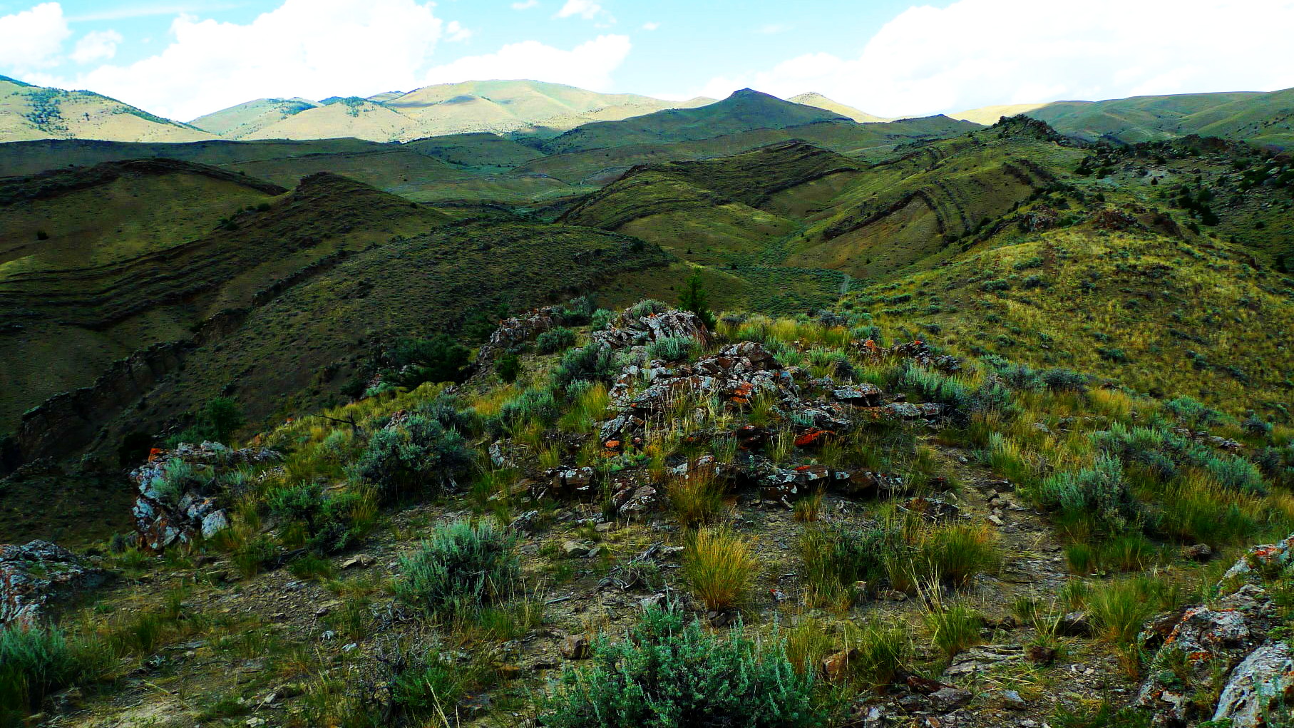
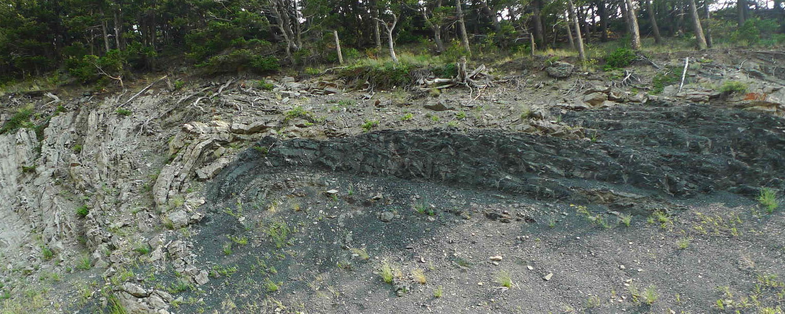
I've been working a bit lately on fluid flow problems involving materials with anisotropic viscosities. That is, deforming such a material in one direction is easier than in another direction. An example of such a material in the real world is a sequence of rock layers with varying strengths. In simple shear along the layered plane the stronger layers are able to slide past each other along the weak layers, but the rock is difficult to squish in "pure shear", because it is supported by the strong layers.

Alternating strong and weak layers in sedimentary rock. Sandy Hollow, MT.

Deformation in layered rock is accommodated primarily in the weak layers. Sun River, MT.

In order to model this sort of behavior I've been working on extending a geodynamic modeling code, aspect, to incorporate more complex constitutive laws. Before I get too far in to ASPECT though I'd like to to step back a bit and define the equations I plan to solve. To that end we can start with the basic governing equations of fluid dynamics.

In general fluid flow obeys the Cauchy momentum equation,

$\rho \frac{D\vec{u}}{Dt} = \nabla \cdot \sigma + \rho \vec{g}$,

where $\vec{u}$ is the fluid velocity field, $\frac{D}{Dt} \equiv \frac{d}{dt} + \vec{u} \cdot \nabla$ is the material derivative, $\sigma$ is the stress tensor, $\rho$ is the fluid density, and $\vec{g}$ is the gravity vector. In geodynamics we deal with very low Reynolds number systems (i.e., momentum is negligibly small), so we set the left hand side of Cauchy's equation to zero. This leaves us with the governing equation:

$-\nabla \cdot \sigma = \rho \vec{g}$.

We often also add the constraint that mass is conserved, $\nabla \cdot (\rho \vec{u}) = 0$, or in some cases that the flow is entirely incompressible, $\nabla \cdot \vec{u} = 0$.

In general, we don't care so much about the stress state of the fluid, but we want to solve for the velocity. Therefore we need an equation to relate applied stress to strain rate. This type of equation is called a "constitutive law," and is dependent on the chemical and state properties of the material. The most general constitutive law can be written in index notation, $\sigma_{ij} = - \overline P \delta_{ij} + C_{ijkl} \varepsilon_{kl}$, where $\overline P$ is the dynamic pressure; $\varepsilon$ is the strain rate, defined as the symmetric component of the gradient of the velocity, $\varepsilon \equiv \frac{1}{2} (\nabla \vec{u} + (\nabla \vec{u})^T)$; and $C_{ijkl}$ is a fourth order tensor, related to the viscosity, which maps strain rates to stresses.

Aspect assumes that the fluid in question is isotropic, and thus reduces to only two values, bulk viscosity (which dissipates energy during compaction and dilation), and shear viscosity which dissipates energy during shear deformation. Further, it is assumed that because bulk viscosity is only important in rapid compressions and dilations, such as sound waves and shock waves, it can be ignored in slow flows like geologic applications. Therefore, in Aspect $C_{ijkl}$ is reduced to a single scalar state variable, $2 \eta$, called the shear viscosity. Generalization back to a full constitutive tensor turns out to be as straightforward as changing the variable type of $\eta$ from a floating point scalar to a symmetric, fourth-order tensor. This modification is easily supported in the finite element library on which Aspect is built. With such a modification it is possible to model any arbitrary constitutive law.

Note (2016/02/16): This draft is already over half a year old, and I've been up to a lot since I wrote it, so I think it's time to just post it and write more in a next installment. For now I'll leave off with some figures to demonstrate the effects of the constitutive law I'm using:

Velocity magnitude is plotted here with velocity vectors overlain. The model setups are the same as in the animated example above except the left and right are stress-free boundaries, and the bottom has a prescribed horizontal velocity to the left. We can see the development of preferred shear directions in the velocity vectors.